Quality of Services

SKI assessment

Knowledge injection methods aim to enhance the sustainability of machine learning by minimizing the learning time required. This accelerated learning can possibly lead to improvements in model accuracy as well. Additionally, by incorporating prior knowledge, the data requirements for effective training may be loosened, allowing for smaller datasets to be utilized. Injecting knowledge has also the potential to increase model interpretability by preventing the predictor from becoming a black-box.

Most existing works on knowledge injection techniques showcase standard evaluation metrics that aim to quantify these potential benefits. However, accurately quantifying sustainability, accuracy improvements, dataset needs, and interpretability in a consistent manner remains an open challenge.

🎯 Standard assessment:

Given:

• an injection procedure $I$,
• some symbolic knowledge $K$,
• a sub-symbolic predictor $N$

We define the “educated” predictor as:

\[\hat{N} = I(K,N)\]

and the standard assessment of this predictor is given by:

\[\epsilon = \pi(\hat{N}) - \pi(N)\]

where $\pi$ is a performance score of choice, i.e. accuracy, MSE, etc.

SKI-Quality of Services

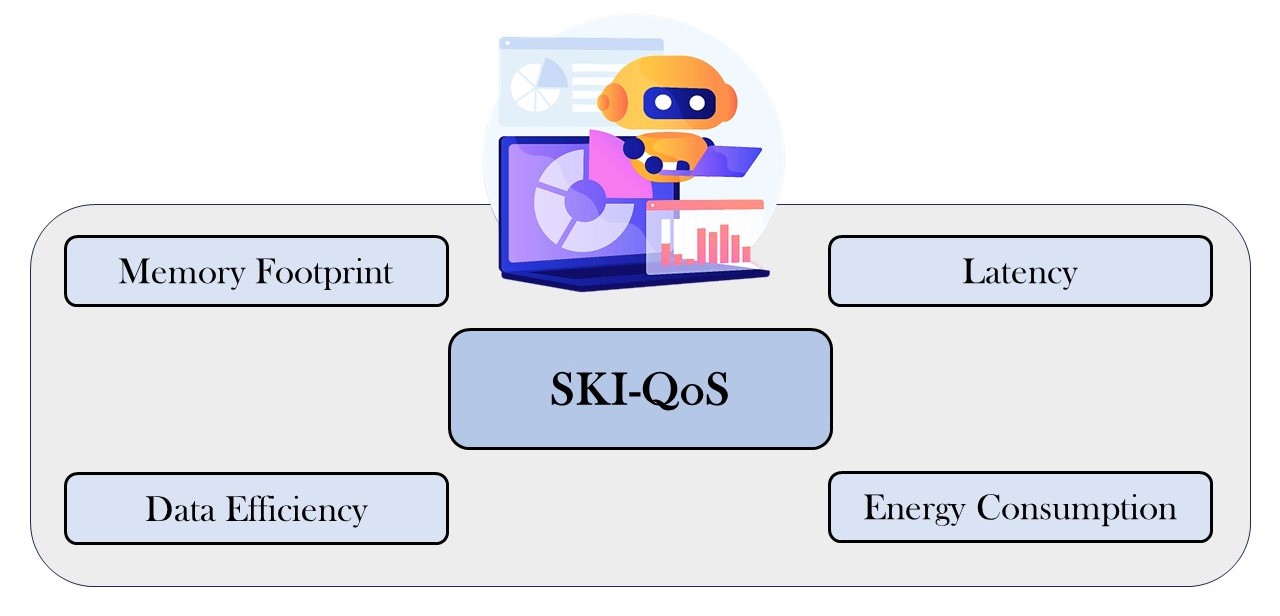
Efficiency metrics:

• Memory footprint, i.e., the size of the predictor under examination;
• Data efficiency, i.e., the amount of data required to train the predictor;
• Latency, i.e., the time required to run a predictor for inference;
• Energy consumption, i.e., the amount of energy required to train/run the predictor;

💾 Memory Footprint

Intuition: injected knowledge can reduce the amount of notions to be learnt data-drivenly.

Idea: measure the amount of total operations (FLOPs or MACs) required by the model.

Formulation:

\[\mu_{\Psi, K, N}(\mathcal{I}) = \Psi(N) - \Psi(\hat{N})\]

where $\hat{N} = \mathcal{I}(K, N)$ represents the educated predictor attained by injecting $K$ into $N$, and $\Psi$ is a memory footprint metric of choice (FLOPs or MACs).

🗂️ Data Efficiency

Intuition: several concepts are injected → some portions of training data are not required.

Idea: reducing the size of the training set $D$ for the educated predictor by letting the input knowledge $K$ compensate for such lack of data.

Formulation:

\[\Delta_\pi(e, N, D, T) = \frac{e}{\pi(N, T)} \sum_{d \in D} \beta(d)\]

where $d$ is a single training sample, $\beta(d)$ is the amount of bytes required for its in-memory representation, and $\pi$ is some performance score of choice.

The data-efficiency gain is equal to:

\[\delta_{e, K, N, D, D', T}(\mathcal{I}) = \Delta_\pi(e, N, D, T) - \Delta_\pi(e, \hat{N}, D', T)\]

⏳ Latency

Intuition: knowledge injection remove unnecessary computations required to draw a prediction.

Idea: measures the average time required to draw a single prediction from a dataset $T$.

Formulation:

\[\Lambda(N, T) = \frac{1}{\vert T \vert} \sum_{t \in T} \Theta(N, t)\]

where $\Theta(N, t)$ represents the time required to draw a prediction from $N$ on the input $t$.

The latency improvement is equal to:

\[\lambda_{K, N, T}(\mathcal{I}) = \Lambda(N, T) - \Lambda(\hat{N}, T)\]

where $\hat{N} = \mathcal{I}(K, N)$ represents the educated predictor attained by injecting $K$ into $N$.

⚡ Energy Consumption

Intuition: knowledge injection reduces learning complexity → reduces amount of computations for training and running a model.

Idea: i) measures the average energy consumption (mW) for a single update, on a training dataset $T$; ii) measures the average energy consumption (mW) of a single forward on a test dataset $T$ composed by several samples.

Formulation:

• Energy consumed by N on a per-single-inference basis:

\[\Upsilon^\mathsf{i}_{\upsilon}(N, T) = \frac{1}{\vert T \vert} \sum_{t \in T} \upsilon(N, t)\]

where $\upsilon(N, t)$ measures the energy consumption of a single forward run of N on a single sample $t$.

• Energy consumed by N during training:

\[\Upsilon^\mathsf{t}_{\upsilon, \gamma}(e, N, T) = \frac{\gamma(e, N, T)}{e \cdot \vert T \vert} - \Upsilon^\mathsf{i}_\upsilon(N, T)\]

where $\gamma(e, N, T)$ measures the overall energy consumed by the training phase as whole.

• The energy consumption improvement is equal to:

\[\varepsilon^\mathsf{i}_{\upsilon, K, N, T}(\mathcal{I}) = \Upsilon^\mathsf{i}_{\upsilon}(N, T) - \Upsilon^\mathsf{i}_{\upsilon}(\mathcal{I}(K, N), T)\] \[\varepsilon^\mathsf{t}_{\upsilon, \gamma, e, K, N, T}(\mathcal{I}) = \Upsilon^\mathsf{t}_{\upsilon, \gamma}(e, N, T) - \Upsilon^\mathsf{t}_{\upsilon, \gamma}(e, \mathcal{I}(K, N), T)\]